Sunday, October 18, 2015

A Guided Genetic Algorithm for the Planning in Lunar Lander Games

A Guided Genetic Algorithm for the Planning in Lunar Lander Games
Zhangbo Liu
Department of Computer Science
University of British Columbia
2366 Main Mall
Vancouver, B.C, V6T 1Z4, Canada
email: zephyr@cs.ubc.ca

KEYWORDS
Guided Genetic Algorithm, Reinforcement Learning,
Planning, Games
ABSTRACT
We propose a guided genetic algorithm (GA) for plan- ning in games. In guided GA, an extra reinforcement component is inserted into the evolution procedure of GA. During each evolution procedure, the reinforcement component will simulate the execution of a series of ac- tions of an individual before the real trial and adjust the series of actions according to the reinforcement thus try to improve the performance. We then apply it to a Lunar Lander game in which the falling lunar module needs to learn to land on a platform safely. We com- pare the performance of guided GA and general GA as well as Q-Learning on the game. The result shows that the guided GA could guarantee to reach the goal and achieve much higher performance than general GA and Q-Learning.
INTRODUCTION
There are two main strategies for solving reinforcement learning problems. The ¯rst is to search in the space of behaviors in order to ¯nd one that performs well in the environment. The second is to use statistical tech- niques and dynamic programming methods to estimate the utility of taking actions in states of the world (Kael- bling et al. 1996). Genetic algorithms (GA) and Tempo- ral Di®erence (TD-based) algorithms (e.g. Q-Learning)belong to each of the two categories, respectively.
Both GA and TD-based algorithms have advantages and disadvantages. GA leads to very good exploration with its large population that can be generated within a gen- eration but weak exploitation with elitism selection op- erator, because its other two operators, the crossover and mutation operators are usually randomly working. TD-based algorithms use two strategies to solve prob- lems with continuous space which are discretization and function approximation. It usually faces the curse of di- mensionality when using discretization. With function approximation it is said to be able to alleviate such a
problem but might be stuck into certain local optima. In this paper, we ¯rst investigate the GA as well as Q- Learning approach on the Lunar Lander game. Then we propose the guided GA by inserting a reinforcement component into the evolution procedure of GA. Since general GA uses random crossover and mutation opera- tions, its performance is quite unstable. Guided GA is designed to achieve higher e±ciency by involving the re- ward concept of reinforcement learning into general GA while keep all components of general GA unchanged so that the extension from general GA to guided GA is easy to achieve.
The remainder of this paper is organized as follows. In section 2 we introduce research work that is relevant to this paper. In section 3 we describe the Lunar Lander game as well as alternative approaches for the problem implemented with general GA and Q-Learning. In sec- tion 4 we present the guided GA approach for the prob- lem. The results of the experiment are shown in section 5 following by the conclusions.
RELATED WORK
Reinforcement Learning for Continuous State- Action Space Problems
The issue of using reinforcement learning to solve contin- uous state-action space problem has been investigated by many researchers. And game is actually an ideal test bed.
There are a few well known benchmark problems in the reinforcement learning domain such as Mountain Car (Moore and Atkeson 1995), Cart-Pole (Barto et al. 1983) and Acrobot (Boone 1997). In the Mountain Car prob- lem, the car must reach the top of the hill as fast as possible and stop there. This problem is of dimension 2, the variables being the position and velocity of the car. The Cart-Pole is a 4-dimensional physical system in which the cart has to go from the start point to the goal and keep the orientation of its pole vertical within a certain threshold when it reaches the goal. The Acrobot problem is also a 4-dimensional problem which consists of a two-link arm with one single actuator at the elbow. The goal of the controller is to balance the Acrobot at
its unstable, inverted vertical position, in the minimum time. Another implementation described in (Ng et al. 2004) made an autonomous inverted helicopter °ight.
Two main strategies here are discretization and func- tion approximation. For the ¯rst strategy, discretization techniques have been widely pursued and provide con- vergence results and rates of convergence (Munos and Moore 2002), (Monson et al. 2004). For the second strategy, several approaches come out on how to con¯g- ure with multiple function approximators (Gaskett et al. 1999), (Smart and Kaelbling 2000).
Reinforcement Learning + Genetic Algorithm
Some researches on combining the advantages of GA and TD-based reinforcement learning have been proposed in (Chiang et al. 1997), (Lin and Jou 1999). However, both of them use gradient decent learning method which is complex and the learning speed is always too slow to achieve the optimum solution. The idea of guided GA we propose is inspired by (Ito and Matsuno 2002), in which Q-Learning is carried out and ¯tness of the genes is calculated from the reinforcedQ-table. However, in guided GA, instead of usingQ-table, we directly insert a reinforcement component into the evolution procedure of the general GA so that the large Q-table and hid- den state problem are avoided. In (Juang 2005), Juang proposed another approach to combine online clustering and Q-valuebased GA for reinforcement fuzzy system design. Compared with the approach described in that paper, guided GA is much simpler in structure and eas- ier to implement while the problem we address in this paper has a higher dimension than that of in (Juang 2005).
THE LUNAR LANDER GAME
The Lunar Lander Game
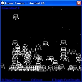
The Lunar Lander game is actually a physically-basedproblem in which the controller needs to gently guide and land a lunar module onto a small landing platform, as shown in Figure 1. The space is a 400 £ 300 pixel rectangle area. It simulates the real environment on the moon that the lunar module has mass and is in°uenced by the gravity on the moon (1.63m/s2). The controller here has 5-dimensional state spaces which are: position (x; y), velocity (x; y) and orientation (µ). The controller is able to do four actions: rotate left, rotate right, thrust and do nothing (drift).
When agent becomes the controller instead human player, the problem becomes to an advanced path ¯nd- ing issue. The successful landing requirement consists the checking of the following variables when any part of the lunar module reach the ground:
² Distance from the pad
Figure 1: The Lunar Lander Game
²Speed
²Degrees of rotation
All of them must be below certain thresholds to achieve safe landing, otherwise it will crash and the game will start from beginning again. The game runs in real time thus it is a good test bed for problems with continuous state and discrete action spaces.
Alternative Approaches
Genetic Algorithm
One alternative approach to this problem is using ge- netic algorithm (GA) for planning. For a complete in- troduction to GA please refer to (Goldberg 1989). The GA approach to this problem follows the steps below in one epoch to try to achieve the goal.
First, the genome is encoded as a series of genes each of which contains an action-duration pair, as shown in Figure 2. The duration here represents the period of time that each speci¯c action is applied. At the begin- ning, all the actions and durations in those genes in one genome are randomly assigned. A number of genomes will be created together in one generation.
Figure 2: Genome encoding
Next, the controller starts a trial according to theaction-duration series in each genome and uses a ¯t- ness function to evaluate their utilities when they crash. There might be many approaches to build the ¯tness
function to this problem. In (Buckland and LaMothe 2002), Buckland and LaMothe suggested the following ¯tness function:
Fitness w¢ disFit w¢ rotFit w¢ airTime (1)
where disFit and rotFit represent the value function of the position and the orientation feature separately. TheairTime is the time period that the lunar module stays in the air which is de¯ned as na=(+ 1) where nis the number of actions it does ignoring the duration and is the velocity at landing. ware the weights that are applied to balance the function. Those weights are quite important and must be carefully decided in order to achieve a good performance. If the safe landing re- quirement is satis¯ed, the ¯tness value will be assigned with a prede¯ned Big Number instead of calculating using the equation (1).
After one trial for all genomes of the current generation, the ¯tness value of each genome will be calculated out and the best genomes with the highest ¯tness value will remain and put into the next generation. Other genomes of the next generation are created by using crossover and mutation operators. The crossover opera- tor works by stepping through each gene in its parents' genome and swapping them at random to generate their o®spring. The mutation operator runs down the length of a genome and alters the genes in both action and duration according to the mutation rate.
The operator will periodically do one epoch after an- other until one genome's result reaches the goal or the number of generations exceeds the prede¯ned maximum value. An implementation of a GA solution to this prob- lem can be found in (Buckland and LaMothe 2002).
Q-Learning
Based on our experience, Q-Learning with only dis- cretization won't work for this problem. So we im- plement a linear, gradient-descent version of Watkins's Q(¸) to this problem with binary features, "-greedy pol- icy, and accumulating traces described in (Sutton and Barto 1998). Tile coding (Sutton and Barto 1998) is also used to partition the continuous space into multi- ple tilings.
THE GUIDED GENETIC ALGORITHM AP- PROACH
The approaches we mentioned in the previous section both have advantages and disadvantages. The GA is simple to implement and is able to achieve the goal, while its disadvantage is that all its actions are randomly assigned so that its performance is quite unstable. The basic concept of Q-Learning approach is also simple and supposed to be e±cient. However, for this game which is a realtimecontinuous-state problem, Q-Learning with
discretization does not work and Q-Learning with func- tion approximation is hard to accommodate. We design the guided GA which incorporates the concept of reward in Q-Learning into GA. Here we call our function "rein- forcement function" because unlike the reward function in Q-Learning whose values need to be summed to cal- culate the Q-value (Prewards), the reinforcement function here gets the immediate ¯tness value and will be extended to ¯tness function at the end of each epoch. In the following subsections we ¯rst introduce the rein- forcement function design for guided GA to this problem then discuss the details of the algorithm.
Reinforcement Function Design
To model the reinforcement function is a very challeng- ing work. It has to be smoothly transformed to the ¯tness function of the general GA (equation (1)) at the end of each epoch so that we can easily extend the gen- eral GA to a guided GA without modifying the existing ¯tness function. On the other hand, it should be prop- erly de¯ned to e±ciently guide the agents to perform better. We tried many di®erent versions until ¯nally reaching a solution.
In equation (1) there are 3 parameters and we need to modify two of them which are disFit and airTime in our reward function. The main di®erence between equation
(1) and the reinforcement function is that in equation (1), all lunar modules reach the ground (position:y = 0) and each of them has an accumulator nwhose value is the number of actions they do during the whole pro- cedure; while in the reinforcement function, the lunar modules are in the air and they only focus on the next action. Based on this di®erence, we build our reinforce- ment function as follows:
We use disFitx to represent disFit in (1), then we builddisFity which is similar to disFitx but for y coordinate. Then our distance function is:
disFits(disFitx)+
(
disFity)2
(2)

wy
where wis used for balancing the weight betweendisFitx and disFity.
airTime, as mentioned in equation (1), is de¯ned as na=(+ 1). In our reinforcement function, nno longer exists, while we ¯nd that a single de¯ned function does not work well all the time since on di®erent stages our focuses might be di®erent. For example, when the lunar module is high in the air we would pay more attention on its horizontal position; while when it is close to the ground it needs to slow down to prepare for landing. So instead of simply rede¯ning it as 1=(+ 1), we take the vertical position into consideration and come with the following de¯nition:
n¤ De¯ning disFitand airTime¤n
if position:y < h1f disFitdisFit£ r; ifposition:y < h2
airTime= 1=(w£ v + 1); gelse airTime= 1=(+ 1);
where hand h(h> h2) are values of height at which we think should change our strategies and wis the weight that can help slow down the velocity of the lunar module to very small values when they nearly reach the ground. is a scaling factor. Then the reward function we build is:
w¢ disFitw¢ rotFit w¢ airTime(3)
where wand rotFit are the same as in (1).
Algorithm Description
In each epoch of the GA, the evolution of its genomes is done by three operators: selection, crossover and mu- tation. The selection is based on elitism, while the crossover and mutation are by random, which leads to the unstable performance of the general GA. In order to better perform the evolution, we insert a reinforce- ment component whose idea comes from the reward in Q-Learning. There are two strategies to do this. The ¯rst one is on-line updating which is similar to other reinforcement learning algorithms. The second one is o®-line updating which updates the whole genome at one time before each epoch. We choose the latter based on the consideration of both the standard mechanism of GA and the real time property of the problem. The high-level description of the guided GA is shown below:
algorithm guided genetic; begin
obtain last generation;
put a few best individuals directly into new generation;
use crossover operator to generate new generation; use mutate operator on the new generation; evolve the new generation;
end
What we add here is the last step whose input is the mutated new generation. Below is the procedure:
procedure evolve; begin
for each individual in the generation
for each gene in i's action-duration series get duration d, current state s;
from state consider all possible actionsa0with duration d, suppose s0are possible resulting states;
select aand sbased on equation (3);
if ssatis¯es safe landing requirement
aà a0; else if a=6 a
aà awith probability (1 ¡ "); update state;
end
where the greedy rate has the same meaning as the"- greedy policy in reinforcement learning. For any given gene of an individual's genome, there are 4 possible ac- tions and numerous durations (in our implementation for the problem the duration ranges from 1 to 30, which means for any given state there are 120 possible states in the next step). And we would only change the action in action-duration pair so that for any given state there are only 4 possible states in the next step.
We use the "-greedy policy here, but unlike the so called greedy genetic algorithm (Ahuja et al. 1995) which fo- cuses on greedy crossover, guided GA is inspired by (Ito and Matsuno 2002) in which the authors used Q-table to integrate Q-Learning with GA. However, for our prob- lem using Q-table won't work because of the large state space. Instead, we use the above method to directly insert the reinforcement component into the evolution procedure without saving any previous state or function value in the memory.
EXPERIMENTAL DETAILS
Experimental Design and Results
We conducted an experiment to test the performance of our guided GA and compared it with the general GA and Q-Learning. For guided GA and general GA, we made all variables the same for both of them to ensure fairness. The parameters of our experiment were given as follows:
1.Both of the two contained 100 individuals in one generation. The maximum number of generations was 500. It supposes to be failed if it did not achieve the goal within 500 generations and then would start from the beginning again. The length of chromosome was 50. The crossover rate was 0.7 and the mutation rate was 0.05. The was 0.1.
2.The thresholds for the safe landing requirements were:
(a)Distance = 10.0
(b)Velocity = 0.5
(c)Rotation = ¼/16
3.To de¯ne the values of weights was the most di±- cult work for the experiment. Below are the best value settings that were selected by empirical study:
(a)w= 1; w= 400; w= 4 (got from (Buckland and LaMothe 2002))
(b) w= 3; w= 6; r = 1:7; h= 100; h= 30
We also introduced the same feature of guided GA toQ-Learning implementation for building its reward func- tion.
To learn to solve a problem by reinforcement learning, the learning agent must achieve the goal (by trial-and-error) at least once (Lin 1992). Testing results showed that general and guided GA were able to achieve the goal almost every time. However, it was very hard forQ-Learning to complete the task. Besides the general reasons such as function approximation strategy often falls into local optimal and Q-Learning converges too slowly, we believed that another important reason was in this realtime problem the control of duration of the action is crucial. GAs could evolve the durations with the crossover and mutation operation. But Q-Learningcould not. Adding duration together with action into the state space might make the state space extremely huge, thus lead to Q-Learning's fail. Based on this fact, we only compared the data we got from the testings using general GA and guided GA. The experimental re- sults that we ran both of general and guided GA for 25 trials are shown in Figure 3.
Figure 3: Experimental Results
From the results we can observe that for most of the time the performance of the guided GA were much higher than the general GA except the last trial. Figure 4 shows the ¯tness that both of them gained during all the generations before the last generation in the 13th trial. According to the data, both the highest and the average ¯tness of guided GA were higher than general GA.
Analysis
Some questions came out when we observed the data of the results. First, what was the goal's ¯t- ness/reinforcement value? Second, why the highest ¯t- ness of guided GA was much higher than that of general GA while they achieved the goal in very close steps? Third, why guided GA lost in the last trial while per- formed much better in previous trials?
Figure 4: Fitness Gained in the 13th Trial
We used the thresholds for the problem to calculate out the ¯tness value and found that the ¯tness value of the goal was just no more than 900. The reason why those individuals with very high ¯tness values failed to achieve the goal was that there were three parameters in the ¯tness/reinforcement function. No matter how high the ¯tness value that certain individual gained, as long as there was one parameter whose value was above the threshold then it failed to achieve the goal. So it was possible that one individual with a low ¯tness achieved the goal in the next generation by randomly evolving its genome which accidentally hit all the thresholds and triggered a sudden success. And that was the reason that sometimes the individual who achieved the goal was not the one who performed the best in the previous state.
Both general and guided GA involved randomness that brought the uncertainty to the procedure. So the possi- ble explanation to the third question was that the ran- domness caused a sudden success to the general GA before the guided GA got out of certain local optimal states.
Although the highest ¯tness in each step did not make much sense to us, the average ¯tness were useful because higher average ¯tness demonstrated a better chance for the whole generation to achieve the goal. For all the trials we observed, the average ¯tness of guided GA were much higher than the average ¯tness of general GA.
CONCLUSION AND FUTURE WORK
In this paper we proposed a guided genetic algorithm by adding a reinforcement component into GA. We success- fully applied the guided GA for the planning of Lunar Lander game. Based on the experimental results, guided GA achieved much higher performance than general GA and Q-Learning.
The guided GA which we proposed in this paper demon- strated very good performance. However, it still has some shortcomings and has the potential to be im- proved. Possible improvement direction are: ¯rst, ¯gure out a method that could update the reinforcement func- tion more e®ectively; second, optimize the procedure of
crossover and mutation; last but not the least, ¯nd out some rules to model the reinforcement function without doing trial-and-error.
ACKNOWLEDGEMENT
We would thank Dr. David Poole, Dr. Michiel van de Panne, Dr. Chris Gaskett and Joel Lanir for their invaluable suggestions on our work. We also appreciate peer reviewers for their precious comments.
REFERENCES
R. Ahuja, J. Orlin, and A. Tivari. A greedy genetic algo- rithm for the quadratic assignment problem. Working pa- per 3826-95, Sloan School of Management, MIT, 1995.
A.G. Barto, R.S. Sutton, and C.W Anderson. Neurolike adaptive elements that can learn di±cult control prob- lems. IEEE. Trans. on System Man and Cybernetics, 1983.
G. Boone. Minimum-time control of the acrobot. Interna- tional Conference on Robotics and Automation, 1997.
M. Buckland and A. LaMothe. AI techniques for game pro- gramming. Premier Press, 2002.
C.K. Chiang, H. Y. Chung, and J. J. Lin. A self-learningfuzzy logic controller using genetic algorithms with rein- forcements. IEEE Transactions on Fuzzy Systems, 1997.
C. Gaskett, D. Wettergreen, and A. Zelinsky. Q-learning in continuous state and action spaces. In Australian Joint Conference on Arti¯cial Intelligence, pages 417{428, 1999.
D.E. Goldberg. Genetic Algorithm in Search, Optimiza- tion and Machine Learning. Kluwer Academic Publishers, 1989.
K. Ito and F. Matsuno. A study of reinforcement learning for the robot with many degrees of freedom - acquisition of locomotion patterns for multi-legged robot. In ICRA '02. IEEE International Conference on Robotics and Au- tomation, pages (4):3392{3397, 2002.
C.F. Juang. Combination of online clustering and q-valuebased ga for reinforcement fuzzy system design. IEEE Transaction on Fuzzy Systems, 2005.
L.P. Kaelbling, M.L. Littman, and A.P. Moore. Reinforce- ment learning: A survey. Journal of Arti¯cial Intelligence Research, 4:237{285, 1996.
C.T. Lin and C.P. Jou. Controlling chaos by ga-based rein- forcement learning neural network. IEEE Transaction on Neural Networks, 1999.
L.J. Lin. Self-improving reactive agents based on reinforce- ment learning, planning and teaching. Mach. Learn., 8(3-4):293{321, 1992.
C.K. Monson, D. Wingate, K.D. Seppi, and T.S. Peterson. Variable resolution discretization in the joint space. In- ternational Conference on Machine Learning and Appli- cations, 2004.
A.W. Moore and C.G. Atkeson. The parti-game algorithm for variable resolution reinforcement learning in multi- dimensional state-spaces. Mach. Learn., 21(3):199{233, 1995.
R. Munos and Andrew Moore. Variable resolution discretiza- tion in optimal control. Mach. Learn.,49(2-3):291{323, 2002.
A.Y. Ng, A. Coates, M. Diel, V. Ganapathi, J. Schulte, B. Tse, E. Berger, and E. Liang. Inverted autonomous helicopter °ight via reinforcement learning, 2004.
W.D. Smart and L.P. Kaelbling. Practical reinforcement learning in continuous spaces. In Proc. 17th International Conf. on Machine Learning, pages 903{910. Morgan Kauf- mann, San Francisco, CA, 2000.
R.S. Sutton and A.G. Barto. Reinforcement Learning: An Introduction. Number 206-214. MIT Press, Cambridge, MA, 1998.
BIOGRAPHY
ZHANGBO LIU studies computer science at the Univer- sity of British Columbia, Canada. His main research in- terests are human-computer interaction and arti¯cial intelli- gence in games.

Saturday, October 17, 2015

Book: Reinforcement Learning: An Introduction

Reinforcement Learning: 

An Introduction 


Richard S. Sutton and Andrew G. Barto
A Bradford Book

The MIT Press
Cambridge, Massachusetts
London, England
In memory of A. Harry Klopf


Mark Lee 2005-01-04

Wednesday, October 14, 2015

A Tutorial for Reinforcement Learning

A Tutorial for Reinforcement Learning
Abhijit Gosavi
Department of Engineering Management and Systems Engineering
Missouri University of Science and Technology
219 Engineering Management, Rolla, MO 65409
Email:gosavia@mst.edu
November 22, 2014
If you find this tutorial useful, or the codes in C at
http://web.mst.edu/~gosavia/bookcodes.html
useful, or the MATLAB codes at
http://web.mst.edu/~gosavia/mrrl_website.html
useful, please do cite my book (for which this material was prepared), now in its second edition.
A. Gosavi. Simulation-Based Optimization: Parametric Optimization Techniques and Re- inforcement Learning, Springer, New York, NY, Second edition, 2014.
Book website: http://web.mst.edu/˜gosavia/book.html
1
Contents
1
Introduction
3
2
MDPs and SMDPs
3
3
RL

6

3.1
Average reward . . . . . . . . . . . . . . . . . . . . . . . . . . . . . . . . . .
7

3.2
Selecting the learning rate or step size . . . . . . . . . . . . . . . . . . . . .
10

3.3
Discounted reward . . . . . . . . . . . . . . . . . . . . . . . . . . . . . . . .
11

3.4
Codes . . . . . . . . . . . . . . . . . . . . . . . . . . . . . . . . . . . . . . .
12
4
Example
12
5
Conclusions
12
2
1Introduction
The tutorial is written for those who would like an introduction to reinforcement learning (RL). The aim is to provide an intuitive presentation of the ideas rather than concentrate on the deeper mathematics underlying the topic.
RL is generally used to solve the so-called Markov decision problem (MDP). In other words, the problem that you are attempting to solve with RL should be an MDP or its variant. The theory of RL relies on dynamic programming (DP) and artificial intelligence (AI). We will begin with a quick description of MDPs. We will discuss what we mean by “complex” and “large-scale” MDPs. Then we will explain why RL is needed to solve complex and large-scale MDPs. The semi-Markov decision problem (SMDP) will also be covered.
The tutorial is meant to serve as an introduction to these topics and is based mostly on the book: “Simulation-based optimization: Parametric Optimization techniques and rein- forcement learning” [3]. The book discusses this topic in greater detail in the context of simulators. There are at least two other textbooks that I would recommend you to read:
(i) Neuro-dynamic programming [1] (lots of details on convergence analysis) and (ii)Rein- forcement Learning: An Introduction [8] (lots of details on underlying AI concepts). A more recent tutorial on this topic is [7]. This tutorial has 2 sections:
Section 2 discusses MDPs and SMDPs.
Section 3 discusses RL.
By the end of this tutorial, you should be able to
Identify problem structures that can be set up as MDPs / SMDPs.
Use some RL algorithms.
We will not discuss how to use function approximation, but will provide some general advice towards the end.
2MDPs and SMDPs
The framework of the MDP has the following elements: (1) state of the system, (2) actions,
(3) transition probabilities, (4) transition rewards, (5) a policy, and (6) a performance metric. We assume that the system is modeled by a so-called abstract stochastic process called the Markov chain. When we observe the system, we observe its Markov chain, which is defined by the states. We explain these ideas in more detail below.
State: The “state” of a system is a parameter or a set of parameters that can be used to describe a system. For example the geographical coordinates of a robot can be used to describe its “state.” A system whose state changes with time is called a dynamicsystem. Then it is not hard to see why a moving robot produces a dynamic system.
Another example of a dynamic system is the queue that forms in a supermarket in front of the counter. Imagine that the state of the queuing system is defined by the number of
3
people in the queue. Then, it should be clear that the state fluctuates with time, and then this is dynamic system.
It is to be understood that the transition from one state to another in an MDP is usually a random affair. Consider a queue in which there is one server and one waiting line. In this queue, the state x, defined by the number of people in the queue, transitions to + 1 with some probability and to − 1 with the remaining probability. The former type of transition occurs when a new customer arrives, while the latter event occurs when one customer departs from the system because of service completion.
Actions: Now, usually, the motion of the robot can be controlled, and in fact we are interested in controlling it in an optimal manner. Assume that the robot can move in discrete steps, and that after every step the robot takes, it can go Northgo South,go East, or go West. These four options are called actions or controls allowed for the robot.
For the queuing system discussed above, an action could be as follows: when the number of customers in a line exceedssome prefixed number, (say 10), the remaining customers are diverted to a new counter that is opened. Hence, two actions for this system can be described as: (1) Open a new counter (2) Do not open a new counter.
Transition Probability: Assume that action is selected in state i. Let the next state be j. Let p(i, a, j) denote the probability of going from state to state under the influence of action in one step. This quantity is also called the transition probability. If an MDP has 3 states and 2 actions, there are 9 transition probabilities per action.
Immediate Rewards: Usually, the system receives an immediate reward (which could be positive or negative) when it transitions from one state to another. This is denoted by r(i, a, j).
Policy: The policy defines the action to be chosen in every state visited by the system. Note that in some states, no actions are to be chosen. States in which decisions are to be made, i.e., actions are to be chosen, are called decision-making states. In this tutorial, by states, we will mean decision-making states.
Performance Metric: Associated with any given policy, there exists a so-called performance metric — with which the performance of the policy is judged. Our goal is to select the policy that has the best performance metric. We will first consider the metric called the average reward of a policy. We will later discuss the metric called average reward. We will assume that the system is run for a long time and that we are interested in a metric measured over what is called the infinite time horizon.
Time of transition: We will assume for the MDP that the time of transition is unity (1), which means it is the same for every transition. Hence clearly 1 here does not have to mean 1 hour or minute or second. It is some fixed quantity fixed by the analyst. For the SMDP, this quantity is not fixed as we will see later.
Let us assume that a policy named π is to be followed. Then π(i) will denote the action selected by this policy for state i. Every time there is a jump in the Markov chain (of the system under the policy in consideration), we say a transition (or jump) has occurred. It is
4
[s=1
important to understand that during a transition we may go from a state to itself!
Let xdenote the state of the system before the sth transition. Then, the following quantity, in which xi, is called the average reward of the policy π starting at state i.
]
r(xs, π(xs), xs+1)|xi
ρ= lim

(1)

k!1
k
This average reward essentially denotes the sum of the total immediate rewards earned divided by the number of jumps (transitions), calculated over a very long time horizon (that is assumes a large value.) In the above, the starting state is and π(xs) denotes the action in state xs. Also note that E[.] denotes the average value of the quantity inside the square brackets.
It is not hard to show that the limit in (1) is such that its value is the same for any value of x1, if the underlying Markov chains in the system satisfy certain conditions (related to the regularity of the Markov chains); in many real-world problems such conditions are often satisfied. Then
ρρ for any value of i.
The objective of the average-reward MDP is to find the policy that maximizes the per- formance metric (average reward) of the policy.
Another popular performance metric, commonly used in the literature, is discounted reward. The following quantity is called the discounted reward of a policy π. Again, let xs
denote the state of the system before the sth jump (transition).


ψklim E k
γ1r(xs, π(xs), xs+1)  xi,
(2)
!1 s=1


where γ denotes the discount factor; this factor, γ, is less than
1 but greater than 0.
Eqn.
(2) has a simple interpretation:
ψ= E[r(x1, π(x1), x2) + γr(x2, π(x2), x3) + γ2r(x3, π(x3), x4) + ···]
The discounted reward essentially measures the present value of the sum of the rewards earned in the future over an infinite time horizon, where γ is used to discount money’s value. We should point out that:
γ (
1
1


1 + µ,
(3)
where µ is the rate of interest; the rate is expressed as a fraction here and not in percent. When µ > 0, we have that 0 < γ < 1. It is worthwhile pointing out that in the MDP, we have 1/(1 + µ) raised to the power 1 because in the MDP we assume a fixed rate of discounting and that the time duration of each transition is fixed at 1. This mechanism thus captures within the MDP framework the notion of time value of money.
The objective of the discounted-reward MDP is to find the policy that maximizes the performance metric (discounted reward) of the policy starting from every state.
Note that for average reward problems, the immediate reward in our algorithms can be earned during the entire duration of the transition. However, for the discounted problems, we will assume that the immediate reward is earned immediately after the transition starts.
5
The MDP can be solved with the classical method of dynamic programming (DP). How- ever, DP needs all the transition probabilities (the p(i, a, j) terms) and the transition rewards (the r(i, a, j) terms) of the MDP.
For Semi-Markov decision problems (SMDPs), an additional parameter of interest is the time spent in each transition. The time spent in transition from state to state under the influence of action is denoted by t(i, a, j). To solve SMDPs via DP one also needs the transition times (the t(i, a, j) terms). For SMDPs, the average reward that we seek to maximize is defined as:


E
[
k

x1
i


s=1 r(xs, π(xs), xs+1)

ρ= lim


|

]
.
(4)


k


k
!1 E


[∑s=1 t(xs, π(xs), xs+1)|xi]

(Technically, lim should be replaced by lim inf everywhere in this tutorial, but we will not worry about such technicalities here.) It can be shown that the quantity has the same limit for any starting state (under certain conditions). A possible unit for average reward here is $ per hour.
For discounted reward, we will, as stated above, assume the immediate reward is earned immediately after the transition starts and does not depend on the duration of the transition. Thus, the immediate reward is a lumpsum reward earned at the start of the transition (when the immediate reward is a function of the time interval, see instead the algorithm in [2]). Also, because of the variability in time, we will assume continuously compounded rate of interest. Then, we seek to maximize:
ψklim [r(x1, π(x1), x2) +
k


s=2
r(xs, π(xs), xs+1)
s+1 e dτ xi]
,
!1


where denotes the discounting factor over a period of length τ (under continuous com- pounding) and τis the time of occurrence of the sth jump (transition). Note that since the immediate reward does not depend on the time τ, it can be taken out of the integral. Essentially, what we have above is the sum of discounted rewards with the discount factor in each transition appropriately calculated using the notion of continuous compounding.
Curses: For systems which have a large number of governing random variables, it is often hard to derive the exact values of the associated transition probabilities. This is called the curse of modeling. For large-scale systems with millions of states, it is impractical to store these values. This is called the curse of dimensionality.
DP breaks down on problems which suffer from any one of these curses because it needs all these values.
Reinforcement Learning (RL) can generate near-optimal solutions to large and complex MDPs. In other words, RL is able to make inroads into problems which suffer from one or more of these two curses and cannot be solved by DP.
3RL
We will describe a basic RL algorithm that can be used for average reward SMDPs. Note that if t(i, a, j) = 1 for all values of i, j,and a, we have an MDP. Hence our presentation will
6
be for an SMDP, but it can easily be translated into that of an MDP by setting t(i, a, j) = 1 in the steps.
It is also important to understand that the transition probabilities and rewards of the system are not needed if any one of the following is true:
1.we can play around in the real world system choosing actions and observing the rewards
2.if we have a simulator of the system.
The simulator of the system can usually be written on the basis of the knowledge of some other easily accessible parameters. For example, the queue can be simulated with the knowledge of the distribution functions of the inter-arrival time and the service time. Thus the transition probabilities of the system are usually not required for writing the simulation program.
Also, it is important to know that the RL algorithm that we will describe below requires the updating of certain quantities (called Q-factors) in its database whenever the system visits a new state.
When the simulator is written in C or in any special package such as ARENA, it is possible to update certain quantities that the algorithm needs whenever a new state is visited.
Usually, the updating that we will need has to be performed immediately after a new state is visited. In the simulator, or in real time, it IS possible to keep track of the state of the system so that when it changes, one can update the relevant quantities.
The key idea in RL is store a so-called Q-factor for each state-action pair in the system. Thus, Q(i, a) will denote the Q-factor for state and action a. The values of these Q-factors are initialized to suitable numbers in the beginning (e.g., zero or some small number to all the Q-factors). Then the system is simulated (or controlled in real time) using the algorithm. In each state visited, some action is selected and the system is allowed to transition to the next state. The immediate reward (and the transition time) that is generated in the transition is recorded as the feedback. The feedback is used to update the Q-factor for the action selected in the previous state. Roughly speaking if the feedback is good, the Q-factor of that particular action and the state in which the action was selected is increased (rewarded) using the Relaxed-SMART algorithm. If the feedback is poor, the Q-factor is punished by reducing its value.
Then the same reward-punishment policy is carried out in the next state. This is done for a large number of transitions. At the end of this phase, also called the learning phase, the action whose Q-factor has the highest value is declared to be the optimal action for that state. Thus the optimal policy is determined. Note that this strategy does not require the transition probabilities.
3.1Average reward
We begin with average reward. The algorithm that we will describe is called R-SMART(Relaxed Semi-Markov Average reward Technique). The original version in [5] required that the average reward be initialized to a value close to its optimal value. We present here a modified version from [4] that does not require this. We first present theCF-version of R- SMART, where CF stands for the contraction factor. We will later present another version
7
of this algorithm.
Steps in CF-version of R-SMART:
The steps in the Learning Phase are given below.
• Step 1: Set the Q-factors to some arbitrary values (e.g. 0), that is:
Q(i, a← 0 for all and a.
Set the iteration count, k, to 1. Let ρdenote the average reward in the kth iteration of the algorithm. Set ρto 0 or any other value. Let the first state be i. Let A(i) denote the set of actions allowed in state i. Let αdenote the main learning rate in the kth iteration. Selecting a value for α (or any learning rate/step size) is a topic that we discuss below. Let βdenote the secondary learning rate. Also set the following two quantities to 0: total reward and total time. IT ERMAX will denote the number of iterations for which the algorithm is run. It should be set to a large number. Set η, a scaling constant, to a small positive value, which is close to but less than 1, e.g., 0.99.
• Step 2: Determine the action associated to the Q-factor that has the highest value in state i. (Imagine there are two actions in a state and their values are Q(i, a) = 19 and Q(i, 2) = 45; the clearly action 2 has the greatest Q-factor.) This is called the greedy action. Select the greedy action with probability (1p(k)), where for instance p(k) could be defined as follows:
G1p(k) = Gk
in which G> G1, and Gand Gare large positive constants, e.g., 1000 and 2000 respectively. With a probability of p(k), choose one of the other actions. This can be done easily. The non-greedy actions are called exploratory actions, and selecting an exploratory action is called exploration. It should be clear that our probability of exploration will decay with k, the iteration number, and it should. (For the two-action case, you can generate a random number between 0 and 1. If the number is less than or equal to (1 − pk), choose the greedy action; otherwise, choose the other action.)
Let the action selected be denoted by a. If is a greedy action, set ϕ = 0 (this means that the action selected is greedy with respect to the Q-factor.) Otherwise, set ϕ = 1. Simulate action a.
• Step 3: Let the next state be denoted by j. Let r(i, a, j) denote the transition reward and t(i, a, j) denote the transition time. Then update Q(i, a) as follows:
Q(i, a)
(1
αQ i, a
) +
αk
r
i, a, j
ρkt
i, a, j
) +
η max Q(j, b.


) (
[
(

(

(j)
]


2A

In the above, maxb2A(jQ(j, b) is essentially the maximum numeric value of all theQ-factors in state j. The value of αshould be selected appropriately. See the next subsection for a discussion on learning rate rules.
8
Step 4: If ϕ = 1, that is the action was non-greedy, go to Step 5. Otherwise, update total reward and total time as follows.
total reward ← total reward + r(i, a, j)total time total time + t(i, a, j).
Then update the average reward as:


ρk+1 ← (1 − βk)ρβ[
total

reward
,


total

time

where β is chosen using a rule that decays to 0 faster than α. The next subsection discusses how appropriate values forα and β can be chosen.
Step 5: Increment by 1. Set: i ← j. If k < ITERMAX, return to Step 2. Otherwise, declare the action for whichQ(i, .) is maximum to be the optimal action for state (do this for all values of i, i.e., for all states to generate a policy), and STOP.
Note that in the above, the exploration probability p(k) gradually decays to 1, and in the limit, the algorithm selects the greedy actions. However, this decay should be gradual. If the decay is very quick (e.g., you use small values for Gand G2), the algorithm will most likely converge to an incorrect solution. In other words, the algorithm should be allowed to explore sufficiently.
Further note: η is a positive scalar selected by the user such that 0 < η < 1. The positive scalar η has to be less than 1; it is the contracting factor (CF) that enables the algorithm to converge gracefully to the optimal solution. Its value should be as close to 1 as possible and should not be changed during the learning. An example could be η = 0.99. For a sufficiently large value ofη, the algorithm is guaranteed to converge to the optimal solution. In practice, η = 1 may also generate convergent behavior, but there is no known proof of this.
The next phase is called the frozen phase because the Q-factors are not updated here. This phase is performed to estimate the average reward of the policy declared by the frozen phase to be the optimal policy. (By optimal, of course, we only mean the best that RL can generate; it may not necessarily be optimal, but hopefully is very similar to the optimal in its performance.) Steps in the Frozen Phase are as follows.
• Step 1: Use the Q-factors learned in the Learning Phase. Set iteration count to 0. IT ERMAX will denote the number of iterations for which the frozen phase is run. It should be set to a large number. Also set the following two quantities to 0: total reward and total time.
Step 2: Select for state the action which has the maximum Q-factor. Let that action be denoted by u. Simulate actionb.
Step 3: Let the next state be denoted by j. Let r(i, u, j) denote the transition reward and t(i, u, j) denote the transition time.
Then update total reward and total time as follows.
total reward ← total reward + r(i, u, j)total time total time + t(i, u, j).
9
Step 4: Increment by 1. Set: ← j. If k < ITERMAX, return to Step 2. Otherwise, calculate the average reward of the policy learned in the learning phase as follows:
ρ total rewardtotal time
and STOP.
The value of ρin the learning phase can also be used as an estimate of the actual ρ while the learning is on. But typically a frozen phase is carried out to get a cleaner estimate of the actual average reward of the policy learned.
Steps in the SSP-version of R-SMART:
We now present the SSP-version of the algorithm, where SSP stands for the stochastic shortest-path problem, a problem that we do not consider in this tutorial. The problem we solve is not an SSP; the algorithm will use a connection to the SSP to solve our average reward problem. Thus, this SSP-version is essentially going to solve the average reward problem that we have considered above. The algorithm’s steps are identical to those of the CF-version described above with two differences:
Step 1: There is no need to select any value for η because η is not needed in this algorithm. Further, choose any state in the system to be a distinguished state, and then denote it by .
The main update in Step 3 will be as follows:
Q i, a
← (1 
αQ i, a
) +
αk
r
i, a, j
ρkt i, a, j
) +
I
j
̸=
i
max Q j, b
.
(
) (
[
(

(
(


(j)
(
)]


2A


In the above, I(≠ ) is the indicator function whose value can be calculated as follows: I(≠ ) = 1 when ≠ and I(≠ ) = 0 when . Note that the indicator function replaces η used in the CF-version.
Note that, in practice, the CF-version of R-SMART often outperforms the SSP-version, although the SSP version can be shown to converge under milder conditions.
3.2Selecting the learning rate or step size
The learning rate (α or β) should be a positive value typically less than 1. It is also a function of k. We need to ensure some conditions on these rules for RL within simulators. These are described in detail in [1]. Some commonly used examples ofstep-sizes are:
αa/(k)
where for instance = 90 and = 100. Another rule is the log rule: log(k)/k (make sure starts at 2; otherwise use log(+ 1)/(+ 1) for starting at 1) studied in [6]. The log rule converges to 0 slower than the a/(k) rule for many values of and b.
10
The rule 1/k where = 1 and = 0 may not lead to good behavior [6], although it is still widely used and was also used by this author in some of his own prior work. (We, obviously, do not recommend it any more, especially after the findings in [6] in the context of Q-Learning).
When we have two step sizes like in R-SMART above, we must make sure that β converges to 0 faster. We can then use α =log(k)/k and β = 90/(100 + k). Ideally, as tends to βkshould tend to 0.
3.3Discounted reward
For discounted reward, the learning phase is sufficient. The steps we describe are from the famous Q-Learning algorithm of Watkins [11]. They apply to the MDP; we will discuss the SMDP extension later.
• Step 1: Set the Q-factors to some arbitrary values (e.g., 0), that is:
Q(i, a← 0 for all and a.
Let A(i) denote the set of actions allowed in state i. Let αdenote the main learning rate in the kth iteration. Set = 1. IT ERMAX will denote the number of iterations for which the algorithm is run. It should be set to a large number.
Step 2: Select an action in state with probability 1/|A(i)|, where |A(i)denotes the number of elements in the set A(i). Simulate action a.
Step 3: Let the next state be denoted by j. Let r(i, a, j) denote the transition reward
and t(i, a, j) denote the transition time. Then update Q(i, a) as follows:
Q i, a
← (1 
αk
Q
i, a
) +
αk
r
i, a, j
) +
γ max Q j, b
,
(
)
(

[
(

(j)
(
)]


2A


where you should compute αusing one of the rules discussed above. Also, γ denotes the discount factor.
Step 4: Increment by 1. Set: ← j. If k < ITERMAX, return to Step 2. Otherwise, for each state declare the action for which Q(i, .) is maximum to be the optimal action, and STOP.
Note that in the algorithm above, there is no decay of exploration. This is because in Q-Learning, the exploration need not decay. However, in practice, to get the algorithm to converge faster, people do employ decay of exploration. It is only recommended in online applications and not in simulators.
For the SMDP extension, you can use the following update in Step 3 of the above algo- rithm (see pages 245-246 of [3] for more details):
Q i, a
← (1 
αk
Q
i, a
) +
αk
r
i, a, j
) +
t(i;a;jmax Q(j, b)
,
(
)
(

[
(

(j)
]


2A

11
where the exponential term arises as follows:

1

γ (
≈ e .

1 + µ
in which τ denotes the time and the discounting mechanism was explained above in Equation
(3). Note that in the above approximation to obtain the exponential term, we use the fact that µ is quite small.
Note on the vanishing discount approach: You can actually use a discounted RL algorithm to solve the average reward problem via the vanishing discount approach. In this heuristic approach, one uses a discounted algorithm with γ very close to 1 (for MDPs) and µ very close to 0 (for SMDPs). This can work very well in practice.
3.4Codes
Some MATLAB codes for these algorithms have been placed on the following website [9]:
http://web.mst.edu/~gosavia/mrrl_website.html
Codes in C have been placed at the following website:
http://web.mst.edu/~gosavia/bookcodes.html
4Example
We end with a simple example from Gosavi [3]. Figure 1 shows a simple MDP; the legend in the figure explains the transition rewards and probabilities. This is an average reward problem on which you could use R-SMART. The optimal policy for this MDP is: action 2 in state 1 and action 1 in state 2. The average reward of the optimal policy is 10.56.
5Conclusions
The tutorial presented above showed you one way to solve an MDP provided you have the simulator of the system or if you can actually experiment in the real-world system. Transition probabilities of the state transitions were not needed in this approach; this is the most attractive feature of this approach.
We did not discuss what is to be done for large-scale problems. That is beyond the scope of this tutorial. What was discussed above is called the lookup-table approach in which each Q-factor is stored explicitly (separately). For large-scale problems, clearly it is not possible to store the Q-factors explicitly because there is too many of them. Instead one stores a few scalars, called basis functions, which on demand can generate the Q-factor for any state-action pair. Function approximation when done improperly can become unstable [3].
We can provide some advice to beginners in this regard. First, attempt to clusterstates so that you obtain a manageable state space for which you can actually use a lookup table.
12
(1,0.7,6)
(2,0.8,13)
(1,0.3,-5)
(2,0.1,17)
1
(1,0.4,7)
2


(2,0.2,-14)

(2,0.9,10)
(1,0.6,12)
Legend:
(a,p,r): a = action
p = transition probability
r = immediate reward
Figure 1: A two state MDP
In other words, divide the state space for each action into grids and use only one Q-factor for all the states in each grid. The total number of grids should typically be a manageable number such as 10000. If this does not work well, produce a smaller number of grids but use an incremental Widrow-Hoff algorithm, that is, a neuron (see [3]), in each grid. If you prefer using linear regression, go ahead because that will work just as well. If this works well, and you want to see additional improvement,do attempt to use neural networks, either neurons or those based on back-propagation [10]. It is with function approximation that you can scale your algorithm up to realistic problem sizes.
I wish you all the best for your new adventures with RL, but cannot promise any help with homework or term papers —sorry :-(
References
[1]D. Bertsekas and J. Tsitsiklis. Neuro-Dynamic Programming. Athena, MA, 1996.
[2]S. J. Bradtke and M. Duff. Reinforcement learning methods for continuous- time Markov decision problems. InAdvances in Neural Information Processing Systems 7. MIT Press, Cambridge, MA, USA, 1995.
[3]A. Gosavi. Simulation-Based Optimization: Parametric Optimization Tech- niques and Reinforcement Learning, Springer, New York, NY, 2014. http://web.mst.edu/˜gosavia/book.html
[4]A. Gosavi. Target-Sensitive Control of Markov and Semi-Markov Processes. Interna- tional Journal of Control, Automation, and Systems9(5):1-11, 2011.
13
[5]A Gosavi. Reinforcement Learning for Long-run Average Cost. European Jour- nal of Operational Research. Vol 155, pp. 654-674, 2004. Can be found at: http://web.mst.edu/˜gosavia/rsmart.pdf
[6]A Gosavi. On Step Sizes, Stochastic Shortest Paths, and Survival Probabilities in Reinforcement Learning, Conference Proceedings of the Winter Simulation Conference, 2009. Available at: http://web.mst.edu/˜gosavia/wsc 2008.pdf.
[7]A Gosavi. Reinforcement Learning: A Tutorial Survey and Recent Advances.INFORMS Journal on Computing. Vol 21(2), pp. 178–192, 2009. Available at: http://web.mst.edu/˜gosavia/joc.pdf
[8]R. Sutton and A. G. Barto. Reinforcement Learning: An Introduction. The MIT Press, Cambridge, MA, USA, 1998.
[9] MATLAB
repository
for

Reinforcement
Learning,

created
by
A.
Gosavi
at
Missouri
University
of
Science
and
Technology,
http://web.mst.edu/˜gosavia/mrrl

website.html.


[10]P. J. Werbos. Beyond regression: New tools for prediction and analysis of behavioral sciences.. Ph.D. thesis, Harvard University, USA, 1974.
[11]C. J. Watkins. Learning from delayed rewards. Ph.D. thesis, Kings College, Cambridge, England, May 1989.
14