Tuesday, December 8, 2015

Learning about deep learning

https://www.lab41.org/learning-about-deep-learning/

GAB41

No. 15
Learning About Deep Learning!

Abhinav Ganesh September 2015PDF Print
With all the coverage on CNN and Fox News lately, Deep Learning has quickly become a household term. Well, not quite, but Deep Learning is definitely all the craze these days for those of us steeped in Machine Learning and big data. We at Lab41 have been trying to find signal in noise over the past few months, and thought it worthwhile to share our “Unauthoritative Practical Getting Started Guide” with others looking to get started with Deep Learning. Before I go on, I must warn you this largely avoids the difficult Greek symbols and other maths underpinning this complex topic. If you’re looking for formal definitions and proofs, you’ll have to follow the links to resources peppered throughout this post. Now let’s get Deeply Learned!

Monday, December 7, 2015

Learning About Deep Learning!

Learning About Deep Learning!

Source:
https://www.lab41.org/learning-about-deep-learning/

No. 15
Learning About Deep Learning!
Abhinav Ganesh September 2015PDF Print
With all the coverage on CNN and Fox News lately, Deep Learning has quickly become a household term. Well, not quite, but Deep Learning is definitely all the craze these days for those of us steeped in Machine Learning and big data. We at Lab41 have been trying to find signal in noise over the past few months, and thought it worthwhile to share our “Unauthoritative Practical Getting Started Guide” with others looking to get started with Deep Learning. Before I go on, I must warn you this largely avoids the difficult Greek symbols and other maths underpinning this complex topic. If you’re looking for formal definitions and proofs, you’ll have to follow the links to resources peppered throughout this post. Now let’s get Deeply Learned!
Why Deep Learning?

Before we get started, we have to ask the most basic question: Why is Deep Learning so interesting?

dog
Photo Credit: TechCrunch
Well, it’s partly because you can be so incredibly flexible and creative with the tasks you want these algorithms to complete:

Andrej Karpathy’s blog post, “The Unreasonable Effectiveness of Recurrent Neural Networks,” provides Deep Learning code to automatically generate text from scratch that looks and reads like Shakespeare. The same code base also can do other impressive things, including generating software source code (in C) that looks like a real programmer wrote it. Pretty soon I’ll probably be out of a job.
People also are starting to write music using neural networks, which lucky for me enabled the extension of my favorite music from the famous song “Let it Go” from Disney’s “Frozen”. It’s amazing; the music actually sounds pretty good, which is incredible since the algorithms did not require human intervention and still managed to learn the rhythm, tempo, and style of the song.
Yarin Gal, a third-year Ph.D. student at Cambridge, was able to take famous pieces of art and extrapolate what the painting would have looked like if the artist had drawn more on the canvas.
These are but a sample of the creative examples posted to places like Hacker News on a seemingly weekly basis, which makes it very exciting how many domains and applications will be improved by this still-bourgeoning field. But the question we asked ourselves is how do we actually get started with understanding deep learning? Since we’re not Ph.D. Machine Learning candidates and don’t work for any of the Google/Facebook/Microsoft brain trusts in the field, we initially felt a bit uneasy about how to tackle the foundations and applications. Luckily for us, people like Karpathy, repos on GitHub, and several other amazing resources are out there if you know where to look. Let’s do just that…

How to Learn about Deep Learning?

As we initially approached this question, we realized that there are already a ton of online resources that can help you get started and we have aggregated many of these resources on our Github Wiki.

Screen Shot 2015-09-17 at 2.22.52 PM

This is great news and shifts the focus from “finding resources” to “filtering good ones.” If you follow down this path, you’ll quickly find that one of the first resources everyone mentions is Andrew Ng’s Coursera class on machine learning (ML).

We found the lectures about basic ML concepts like linear and logistic regression to be useful if you don’t have much of a ML background. More specific to Deep Learning, we found the lectures on neural networks to be a great primer for understanding the basic concepts and architectures. Once we got a hang of some of the basic neural net lingo we found a lecture series that Quoc Le (from the Google Brain project) gave at Carnegie Mellon a few years ago to be very effective. That lecture series not only explains what neural networks are, but also shows examples of how a place like Google uses them and why we call this field “deep learning”.

Screen Shot 2015-09-17 at 4.43.47 PM

After we watched these different lecture series’, we felt like we were getting a grasp of the field. However, we were still looking for something that tied the math and theory to a practical application in a cohesive way. One of the best resources we evaluated for putting this picture together were the notes by the aforementioned Andrej Karpathy for his class at Stanford “Convolutional Neural Networks for Visual Recognition”. His notes are tremendously clear and understandable (unlike many other deep learning texts we found) and explain how to think of complicated deep learning concepts in simpler terms. We really can’t emphasize enough how his notes (which led us to referring to him as Andrej the Jiant) illuminated so many difficult topics and helped us transition from “reading about” to “actually doing” Deep Learning.

Photo Credit: Stanford University

Once we got a good sense for the overall picture with a combination of class notes and lecture videos, we were in a good position to start understanding recent academic literature in this space. We found the transition from more high-level resources like Andrew Ng’s class to more specific example based resources like Andrej Karpathy’s notes to be extremely valuable in solidifying our understanding of key concepts. As we alluded to earlier, the resources mentioned above represent only a
few
of the resources we used to get started. More detailed resources lists can be found on our Github Wiki, which includes deep learning textbooks and academic papers we’re reading that apply deep learning in interesting domains.

Next Steps

So where do we plan to go from here? We’ve seen great progress in the computer vision field with people getting higher and higher scores on ImageNet. This is great news for the field and for image-related applications. However, as a recent Nature article from Bengio, Hinton, and LeCun highlighted, Natural Language Processing could be the next frontier to benefit from Deep Learning architectures. Classes like Richard Socher’s at Stanford, “Deep Learning for Natural Language Processing” (the class notes and lectures are freely available!) only reinforce this notion and indicate the growing interest in this area.

Photo Credit: Stanford University

Since text processing is central to so many of our challenges at Lab41, we wanted to use NLP as our first hands-on foray into the field. Stay tuned to our blog as we document our exploration of Deep Learning! Our journey will be documented in code and Wiki within our Github repository and with blog entries centered on the following topics:

Deep Learning applied to text: Sentiment analysis vs. Traditional ML approaches
Easy setup of development environment for Deep Learning using Docker and GPU’s
Deep Learning framework comparison: Theano vs Caffe vs Torch vs What is a Keras?


Contact us at info@lab41.org
© 2015

In-Q-Tel
 

2 New first steps - AI projects to study

Neural Slime Volleyball


neural_slime_volleyball
Recurrent neural network playing slime volleyball.  Can you beat them?
I remember playing this game called slime volleyball, back in the day when Java applets were still popular.  Although the game had somewhat dodgy physics, people like me were hooked to its simplicity and spent countless hours at night playing the game in the dorm rather than getting any actual work done.
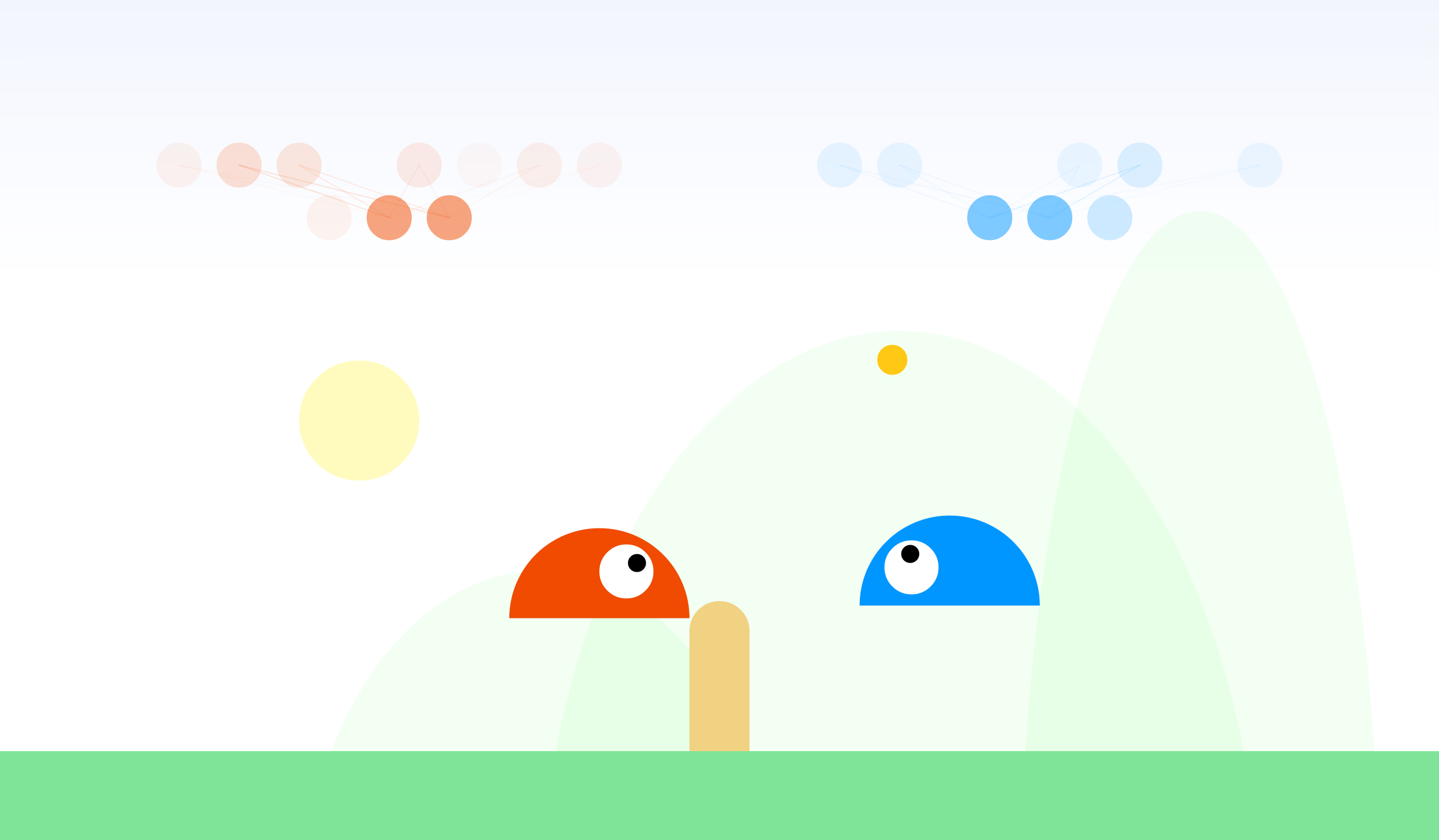
As I can’t find any versions on the web apart from the old antiquated Java applets, I set out to create my own js+html5 canvas based version of the game (complete with the unrealistic arcade-style ‘physics’).  I set out to also try to apply the genetic algorithm coded earlier to train a simple recurrent neural network to play slime volleyball.  Basically, I want to find out whether even a simple conventional neuroevolution techniques can train a neural network to become an expert at the this game, before exploring more advanced methods such as NEAT.
The first step was to write a simple physics engine to get the ball to bounce off the ground, collide with the fence, and with the players.  This was done using the designer-artist-friendly p5.js library in javascript for the graphics, and some simple physics math routines.  I had to brush up the vector maths to get the ball bouncing function to work properly.  After this was all done, the next step was to add in keyboard / touchpad so that the players can move and jump around, even when using a smartphone / tablet.
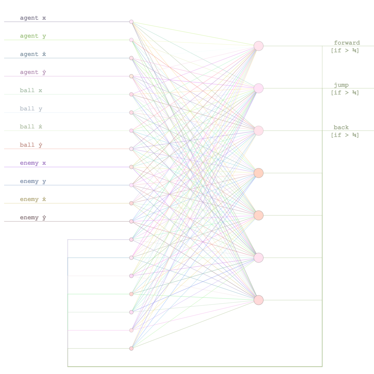
The fun and exciting part was to create the AI module to control the agent, and to see whether it can become good at playing the game.  I ended up using basic CNE method implemented earlier, as an initial test, to train a standard recurrent neural network, hacked together using the convnet.js library.  Below is a diagram of the recurrent network we will train to play slime volleyball, where the magic is done:
slime_rnn
The inputs of the network would be the position and velocity of the agent, the position and velocity of the ball, and also of the opponent.  The output would be three signals that would trigger the ‘forward’, ‘backward’, and ‘jump’ controls to be activated.  In addition, an extra 4 hidden neurons would act as hidden state and fed back to the input, this way it is essentially an infinitely deep feed forward neural network, and potentially remember previous events and states automatically in the hopes of being able to formulate more complicated gameplay strategies.  One thing to note is that the activation functions would fire only if the signal is higher than a certain threshold (0.75).
I also made the agent’s states be the same independent of whether the agent was playing on the left or the right hand side of the fence, by having their locations be relative to the fence, and the ball positions adjusted accordingly according to which side they were playing in.  That way, a trained agent can use the same neural network to play on either side of the fence.
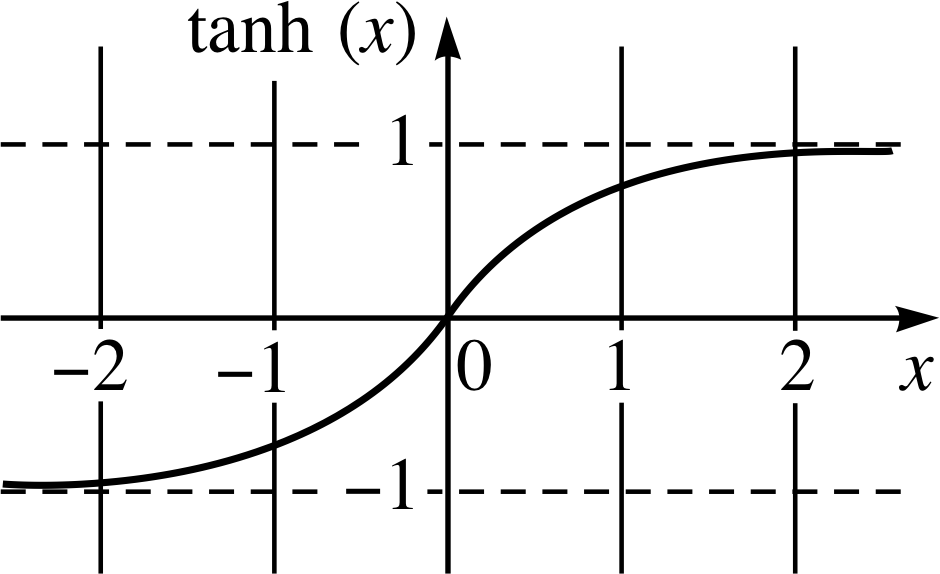
Rather than using the sigmoid function, I ended up using the hyperbolic tangent (tanh) function to control the activations, which convnet.js supports.
The tanh function is defined as:
tanh
The tanh function can be a reasonable activation function for a neural network, as it tends towards +1 or -1 when the inputs get steered one way or the other.  The x-axis would be the game inputs, such as the locations and velocities of the agent, the ball, and the opponent (all scaled to be +/- 1.0 give or take another 1.0) and also the output and hidden states in the neural network (which will be within +/- 1.0 by definition).
tanh_graph
As velocities and ball locations can be positive or negative, this may be more efficient and a more natural choice compared to the sigmoid.  As explained earlier, I also scaled my inputs so they were all in the order of +/- 1.0 size, similar to the output states of the hidden neurons, so that all inputs to the network will have roughly the same orders of magnitude in size on average.
Training such a recurrent neural network involves tweaks on the genetic algorithm trainer I made earlier, since there’s really no fitness function that can return a score, as either one wins or loses a match.  What I ended up doing is to write a similar training function that gets each agent in the training population to play against other agents.  If the agent wins, its score increases by one, and decreases by one if it loses.  On ties (games that longer than the equivalent of 20 real seconds in simulation), no score is added or deducted.  Each agent will play against 10 random agents in the population in the training loop.  The top 20% of the population is kept, the rest discarded, and crossover and mutations are performed for the next generation.  This is referred to as the ‘arms race’ method to train agents to play a one-on-one game.
By using this method, the agents did not need to be programmed by hand any heuristics and rules of the game, but will simply explore the game and figure out how to win.  And the end result suggests that they seem to be quite good at it, after a few hundred generations of evolution!  Check out the demo of the final result below on the youtube video.

The next step can be employ more advanced methods such as NEAT, or ESP for the AI, but that can be overkill for a simple pong-line game.  It is also a candidate for applying the Deep Q-Learner already built in convnetjs, as the game playing strategy is quite simple.  For now I think I have created a fairly robust slime volleyball player that is virtually impossible to beat by a human player consistently.
Try the game out yourself and see if you can beat it consistently.  It works on both desktop (keyboard control), or smartphone / tablet via touch controls.  Desktop version is easier to control either via keyboard arrows or mouse dragging.  Feel free to play around with the source on github, but apologies if it’s not the neatest structured code as it is intended to be more of a sketch rather than a proper program.
Update (13-May-2015)
This demo at one point got to the front page of Y Combinator’s Hacker News.  I made another demo showing the evolution of Agent’s behaviour over time, from knowing nothing at the beginning.  Please see this post for more information.


========================================================================


dlib C++ Library

 Reinforcement Learning, Control, and 3D Visualization

source: http://blog.dlib.net/2015/06/reinforcement-learning-control-and-3d.html?m=0


Over the last few months I've spent a lot of time studying optimal control and reinforcement learning. Aside from reading, one of the best ways to learn about something is to do it yourself, which in this case means a lot of playing around with the well known algorithms, and for those I really like, including them into dlib, which is the subject of this post.  So far I've added two methods, the first, added in a previous dlib release was the well known least squares policy iteration reinforcement learning algorithm.  The second, and my favorite so far due to its practicality, is a tool for solving model predictive control problems.

There is a dlib example program that explains the new model predictive control tool in detail.  But the basic idea is that it takes as input a simple linear equation defining how some process evolves in time and then tells you what control input you should apply to make the process go into some user specified state.  For example, imagine you have an air vehicle with a rocket on it and you want it to hover at some specific location in the air.  You could use a model predictive controller to find out what direction to fire the rocket at each moment to get the desired outcome.  In fact, the dlib example program is just that.  It produces the following visualization where the vehicle is the black dot and you want it to hover at the green location.  The rocket thrust is shown as the red line:


// The contents of this file are in the public domain. See LICENSE_FOR_EXAMPLE_PROGRAMS.txt
/*
This is an example illustrating the use of the linear model predictive
control tool from the dlib C++ Library. To explain what it does, suppose
you have some process you want to control and the process dynamics are
That is, the next state the system goes into is a linear function of its
described by the linear equation: x_{i+1} = A*x_i + B*u_i + C
current state (x_i) and the current control (u_i) plus some constant bias or disturbance.
drive the state (x) to some reference value, which is what we show in this
A model predictive controller can find the control (u) you should apply to example. In particular, we will simulate a simple vehicle moving around in
*/
a planet's gravity. We will use MPC to get the vehicle to fly to and then hover at a certain point in the air.
#include <dlib/gui_widgets.h>
#include <dlib/control.h>
#include <dlib/image_transforms.h>
using namespace std;
using namespace dlib;
// ----------------------------------------------------------------------------
int main()
{
const int STATES = 4;
const int CONTROLS = 2;
// The first thing we do is setup our vehicle dynamics model (A*x + B*u + C).
// Our state space (the x) will have 4 dimensions, the 2D vehicle position
// and also the 2D velocity. The control space (u) will be just 2 variables
// which encode the amount of force we apply to the vehicle along each axis.
// Therefore, the A matrix defines a simple constant velocity model.
matrix<double,STATES,STATES> A;
A = 1, 0, 1, 0, // next_pos = pos + velocity
0, 1, 0, 1, // next_pos = pos + velocity
0, 0, 1, 0, // next_velocity = velocity
0, 0, 0, 1; // next_velocity = velocity
// Here we say that the control variables effect only the velocity. That is,
// the control applies an acceleration to the vehicle.
matrix<double,STATES,CONTROLS> B;
B = 0, 0,
0, 0,
1, 0,
0, 1;
// Let's also say there is a small constant acceleration in one direction.
// This is the force of gravity in our model.
matrix<double,STATES,1> C;
C = 0,
0,
0,
0.1;
const int HORIZON = 30;
// Now we need to setup some MPC specific parameters. To understand them,
// let's first talk about how MPC works. When the MPC tool finds the "best"
// control to apply it does it by simulating the process for HORIZON time
// steps and selecting the control that leads to the best performance over
// the next HORIZON steps.
//
// To be precise, each time you ask it for a control, it solves the
// following quadratic program:
//
// min sum_i trans(x_i-target_i)*Q*(x_i-target_i) + trans(u_i)*R*u_i
// x_i,u_i
//
// such that: x_0 == current_state
// x_{i+1} == A*x_i + B*u_i + C
// lower <= u_i <= upper
// 0 <= i < HORIZON
//
// and reports u_0 as the control you should take given that you are currently
// in current_state. Q and R are user supplied matrices that define how we
// penalize variations away from the target state as well as how much we want
// to avoid generating large control signals. We also allow you to specify
// upper and lower bound constraints on the controls. The next few lines
// define these parameters for our simple example.
matrix<double,STATES,1> Q;
// Setup Q so that the MPC only cares about matching the target position and
// ignores the velocity.
Q = 1, 1, 0, 0;
matrix<double,CONTROLS,1> R, lower, upper;
R = 1, 1;
lower = -0.5, -0.5;
upper = 0.5, 0.5;
// Finally, create the MPC controller.
mpc<STATES,CONTROLS,HORIZON> controller(A,B,C,Q,R,lower,upper);
// Let's tell the controller to send our vehicle to a random location. It
// will try to find the controls that makes the vehicle just hover at this
// target position.
dlib::rand rnd;
matrix<double,STATES,1> target;
target = rnd.get_random_double()*400,rnd.get_random_double()*400,0,0;
controller.set_target(target);
// Now let's start simulating our vehicle. Our vehicle moves around inside
// a 400x400 unit sized world.
matrix<rgb_pixel> world(400,400);
image_window win;
matrix<double,STATES,1> current_state;
// And we start it at the center of the world with zero velocity.
current_state = 200,200,0,0;
int iter = 0;
while(!win.is_closed())
{
// Find the best control action given our current state.
matrix<double,CONTROLS,1> action = controller(current_state);
cout << "best control: " << trans(action);
// Now draw our vehicle on the world. We will draw the vehicle as a
// black circle and its target position as a green circle.
assign_all_pixels(world, rgb_pixel(255,255,255));
const dpoint pos = point(current_state(0),current_state(1));
const dpoint goal = point(target(0),target(1));
draw_solid_circle(world, goal, 9, rgb_pixel(100,255,100));
draw_solid_circle(world, pos, 7, 0);
// We will also draw the control as a line showing which direction the
// vehicle's thruster is firing.
draw_line(world, pos, pos-50*action, rgb_pixel(255,0,0));
win.set_image(world);
// Take a step in the simulation
current_state = A*current_state + B*action + C;
dlib::sleep(100);
// Every 100 iterations change the target to some other random location.
++iter;
if (iter > 100)
{
iter = 0;
target = rnd.get_random_double()*400,rnd.get_random_double()*400,0,0;
controller.set_target(target);
}
}
}
// ----------------------------------------------------------------------------